Who Bit Whom?

Positional Encoding, Explained From First Principles

The Bug Report

Imagine you’re handed a bug report. The system in question is a language model, and someone has filed this ticket:

Bug: Model cannot distinguish “The dog bit the man” from “The man bit the dog.” Treats both sentences as functionally identical.

Your first instinct as an engineer is probably: that’s not a bug, that’s a catastrophic design flaw. Those two sentences share every single word. They differ only in arrangement. And yet the arrangement is the entire point — one is a boring Tuesday, the other is front-page news.

So you go digging into the codebase. And here’s what you find, which should feel deeply wrong to you as a programmer: the model doesn’t read the sentence left to right. It doesn’t process a queue. It doesn’t even process a list. Every word gets converted to a vector, and then — because Transformers are built for speed — all of those vectors get processed simultaneously, in parallel, all at once.

If you’ve written code, you know exactly what data structure that resembles.

“Wait,” you might say, “if it’s processing everything at once with no notion of sequence... isn’t that basically dumping my sentence into some unordered container instead of a list()?”

Yes. Exactly that. Consider what happens if you tally the words in collections.Counter — a frequency dictionary:

>>> from collections import Counter
>>> Counter(["the", "dog", "bit", "the", "man"])
Counter({'the': 2, 'dog': 1, 'bit': 1, 'man': 1})

The words are all there. The counts are perfectly preserved — "the" really did show up twice. But the timeline is gone. There’s no way to rebuild the original sentence from that dictionary; Counter({'the': 2, 'dog': 1, 'bit': 1, 'man': 1}) is equally consistent with “the dog bit the man” and with a dozen other orderings that make no sense at all. That’s the shape of the problem — not that information vanishes, but that sequence specifically vanishes while everything else survives.

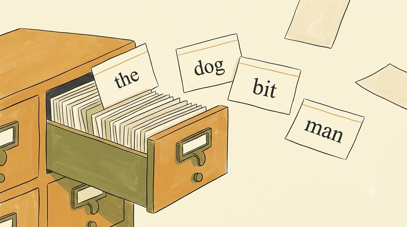
That’s the actual bug. And it’s not a bug someone forgot to fix — it’s the direct, unavoidable side effect of the thing that makes Transformers fast in the first place. Older models (RNNs) did preserve order, because they read one word at a time, carrying a memory forward, the way you’d walk through a linked list one node at a time. But that sequential walk is slow, and it’s exactly why RNNs struggled to train on huge amounts of text. Transformers threw the sequential walk away to get speed. Which means somebody has to reintroduce “order” as an explicit piece of data, since it’s no longer implicit in how the machine reads.

“Okay, so why not just tag each word with its index? word_0, word_1, word_2... Problem solved, right?”

Good instinct. That’s the obvious first fix. Let’s see why it doesn’t survive contact with reality.

Why the Obvious Fix Fails

Say you append a plain integer to each word vector: position 0, 1, 2, 3... What goes wrong?

Problem one — scale. Your embedding values are small, carefully-trained numbers, roughly in the range of -1 to 1. Now you’re appending a raw integer that could be 400 or 4,000 depending on how long the document is. That integer will completely dominate the vector. It’s like trying to average someone’s shoe size with their net worth — one number swamps the other.

Problem two — generalization. The model gets trained on sentences of, say, up to 500 tokens. Then in production someone feeds it a document with 3,000 tokens. Position “2,847” is a number the model has never seen during training. It has no idea what to do with it. A raw index doesn’t generalize past whatever range it was trained on — you’ve baked a hard ceiling into the architecture.

Problem three — no sense of “nearness.” Here’s the sharper version of this problem. It’s not that a raw index is a bad measure of distance on its own — subtraction would work fine. The problem is how the model actually uses it. Attention doesn’t subtract positions. It computes dot products. If the raw position number sat in one dimension of the Query and Key vectors, that dimension’s contribution to the attention score would be pos_Q × pos_K — a product, not a difference. Watch what that does:

pos 5   × pos 6   = 30
pos 500 × pos 501 = 250,500
pos 5   × pos 501 = 2,505

Position 5 and position 6 are neighbors — as close as two tokens can be. Position 5 and position 501 are almost 500 words apart. But the product for the far-apart pair (2,505) is larger than the product for the neighboring pair (30). Multiplication doesn’t preserve “closeness” — it preserves magnitude. Feed a raw integer into the kind of math attention actually does, and it tells the model almost nothing about proximity.

So the fix needs to satisfy three constraints at once: stay small and well-behaved like the embeddings it sits next to, generalize to sequence lengths never seen during training, and encode “nearness” in a way the model’s math can actually exploit.

This is where it gets genuinely clever.

The Odometer

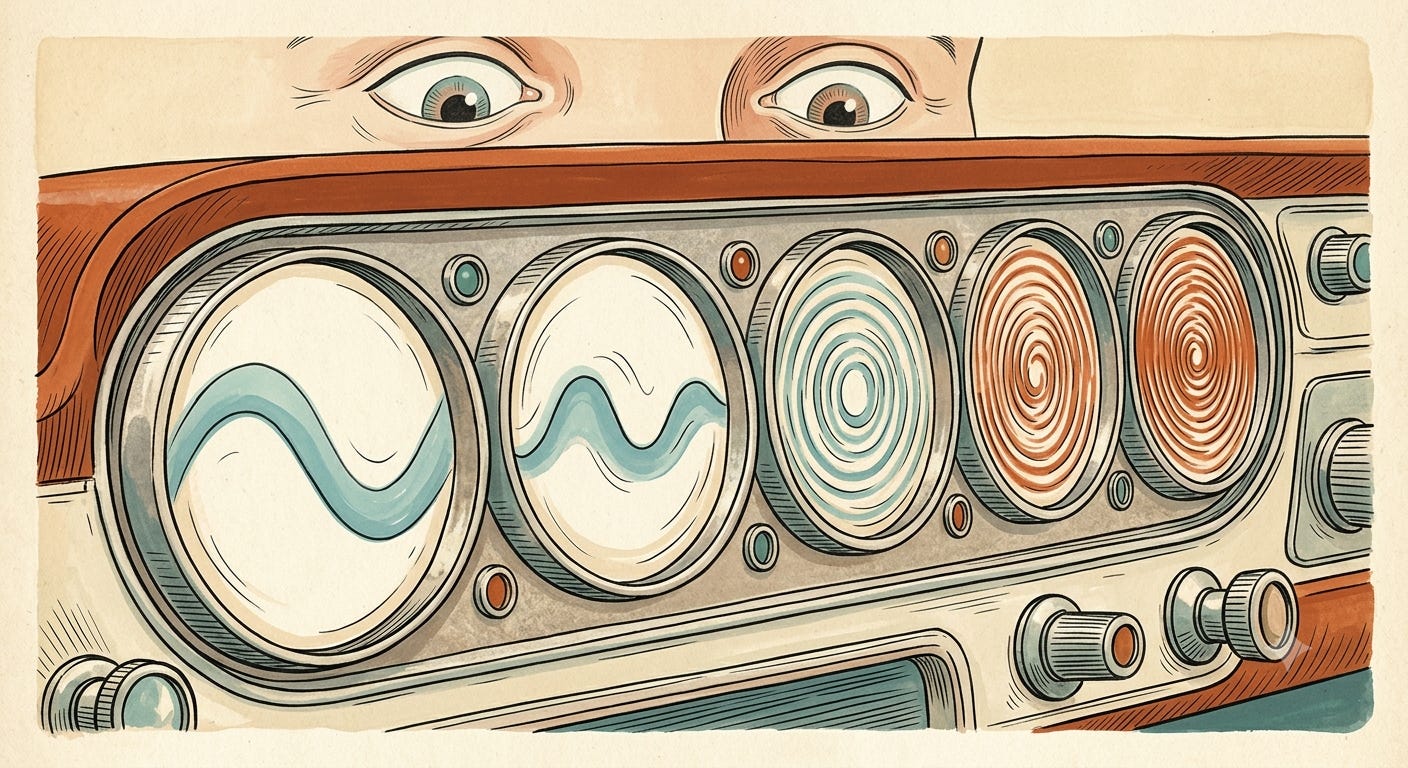
Picture a car odometer — the mechanical kind with several dials side by side. The rightmost dial (ones) spins fast: it ticks over with every mile. The dial to its left (tens) spins ten times slower. The one after that (hundreds) is slower still.

No single dial tells you the mileage. But read together, the combination of all the dials uniquely identifies any mileage number, from 1 to 999,999. And here’s the important part: two mileages that are close together — say, 4,821 and 4,823 — look almost identical on the odometer. Only the fastest dial has moved. Two mileages that are far apart — 4,821 and 891,204 — look totally different across every dial.

That’s the entire trick behind positional encoding. Instead of one dial spinning at one speed, the Transformer gives every position a set of “dials” — except instead of mechanical wheels, they’re waves. Some waves oscillate very fast (they distinguish position 5 from position 6). Some oscillate very slowly (they distinguish “somewhere near the start” from “somewhere near the end,” even across a 4,000-word document). Read together, the combination of wave-values at any position is like a unique barcode for that position — a fingerprint no other position shares.

“Okay, but why waves specifically? Why not just use a bunch of different-speed counters, like the odometer, and skip the trigonometry?”

Because counters reset and clip — they’re not smooth, and they don’t have a mathematical property we’re about to need. Waves do. Stick with me for one more step and it’ll click.

Why Sine and Cosine, Specifically

Here’s the piece that makes this more than a cute analogy. There’s a basic trigonometric identity you probably haven’t touched since school:

The sine and cosine of (A + B) can be computed as a simple linear combination of the sine and cosine of A and of B.

You can try to derive the formula for Sin(A+B) using this diagram

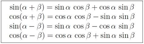
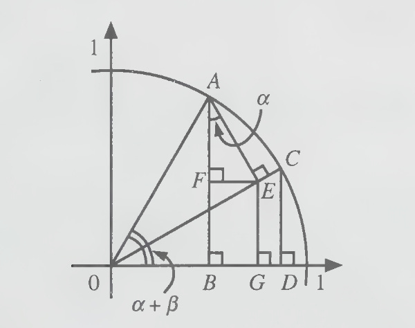
In plain English: if you know the wave-values at one position, you can get the wave-values at any nearby position using a simple, fixed rotation — not by looking anything up, not by memorizing a table, just a small linear transformation, the mathematical equivalent of turning a dial by a fixed number of degrees.

Why does the model care about that? Because attention is fundamentally about relationships between positions — “the word three positions to my left,” “the subject earlier in this sentence.” If relative position can be expressed as a simple rotation, the model can learn one general-purpose “look three words back” operation and reuse it everywhere in the sequence, instead of learning a completely separate rule for every possible pair of absolute positions. That’s the difference between writing one clean function and hardcoding ten thousand special cases.

“So it’s not really about the wave shape at all — it’s about the wave shape making relative offsets cheap to compute?”

Exactly. The odometer analogy gets you the intuition (multiple speeds, combined, make a unique fingerprint). The trig identity is why waves specifically were chosen over, say, sawtooth counters — they’re the one shape that turns “how far apart are these two positions” into arithmetic the network can learn easily.

Putting a Name to It

Before writing the formula, it helps to define its variables one at a time — the way you’d declare variables at the top of a script before writing the function that uses them. There are three, and each answers a different question.

1. The canvas — d

Question: how big is the row we’re filling in?

The positional encoding for one word is just a row of empty slots — d of them. For a small example with d = 8:

slot:  [0]  [1]  [2]  [3]  [4]  [5]  [6]  [7]
value: [ ]  [ ]  [ ]  [ ]  [ ]  [ ]  [ ]  [ ]

d has almost nothing to do with positional encoding specifically — it’s the width of every vector in the model: word embeddings, Query/Key/Value vectors, all of it. Positional encoding just has to match that width, because it gets added directly on top of the word embedding, slot for slot — you can’t add an 8-slot vector to a 6-slot one any more than you can add two arrays of different lengths in code. Whatever width the rest of the model uses, this vector inherits.

The people designing the model pick that width once, before training starts — a hyperparameter, the same category of decision as “how many hidden units in this layer.” Bigger d gives each word more numbers to describe its meaning with, but every weight matrix touching that vector grows with it too — more memory, more compute, at every layer, for every word. The original Transformer paper landed on d = 512 for its base model by experimenting — trying sizes, measuring quality against cost. Modern large models use several thousand. Nobody derived the number from a formula; it’s tuned like any other hyperparameter. The 8 used here is smaller still, chosen for one reason only: so the table coming up fits on a screen.

Critically: d is fixed at design time and never changes. It isn’t a property of any one sentence — it’s baked into the shape of every weight matrix in the model, fixed the moment training begins. A matrix trained expecting 8 numbers in breaks the instant you hand it 6. So d can’t “flex” per sentence, bigger for a long paragraph and smaller for a short one.

2. The location — pos

Question: which word are we filling this row in for?

That’s pos — just the index of the word in the sentence. “Dog” in “the dog bit the man” might be pos = 1. Nothing complicated: pos is simply “which word.”

The key thing that distinguishes pos from d: pos has no upper limit. It isn’t capped by d at all — it’s just whatever index a word lands on, and it can be 5, or 500, or 50,000, because sine and cosine don’t have an upper bound the way an array index does. It grows for as long as the document does. Keep this distinction in mind as we go — d is fixed once and forever; pos is different for every word and can grow arbitrarily large.

3. The dials — i

Question: within that row, how do we actually decide what value goes in each slot?

Two slots at a time. Each pass fills one adjacent pair — one sine value, one cosine value — at a particular speed, then moves on to the next pair at a different, slower speed. That counter — which pair we’re currently filling — is i. i = 0 fills slots 0 and 1 at the fastest speed. i = 1 fills slots 2 and 3, slower. And so on, until the row is full. Since every i fills exactly 2 slots, an 8-slot row needs exactly 4 values of i — d/2 in general.

slot: [0] [1] [2] [3] [4] [5] [6] [7]

value: -0.959 0.284 0.479 0.878 0.050 0.999 0.005 1.000

└─ i=0 ─┘ └─ i=1 ─┘ └─ i=2 ─┘ └─ i=3 ─┘

(sin, cos) (sin, cos) (sin, cos) (sin, cos)

Why sine and cosine together, instead of just one value per pair? Because a single sine value is ambiguous — sin(30°) and sin(150°) are both 0.5, so one number can’t tell you which angle you’re actually at. Sine and cosine together pin the angle down exactly, the same way an (x, y) coordinate pins down one exact point on a circle. So each pair is really “the exact position of a point rotating around a circle at this pair’s particular speed” — and the two coordinates for that point get stored in the pair’s two adjacent slots.

Like d, the number of pairs (d/2) is fixed once, at design time, because this vector has to line up slot-for-slot with the word embedding it gets added to. Nobody adds more pairs because today’s document happens to be long — that job belongs entirely to pos, which we just said has no ceiling. The number of dials is fixed; how far you can spin them isn’t.

The table

With all three variables defined, here’s what actually comes out of this process, for positions 5, 6, and 305:

pos sin,cos (i=0) sin,cos (i=1) sin,cos (i=2) sin,cos (i=3)

5 -0.959, 0.284 0.479, 0.878 0.050, 0.999 0.005, 1.000

6 -0.279, 0.960 0.565, 0.825 0.060, 0.998 0.006, 1.000

…

…

305 -0.262, -0.965 -0.793, 0.609 0.092, -0.996 0.300, 0.954

Position 5 → 6, a single step: the i=0 column swings hard, from (-0.96, 0.28) to (-0.28, 0.96) — that’s the fast pair.

The i=3 column barely moves, (0.005, 1.000) to (0.006, 1.000) — the slow pair.

Position 5 → 305, a 300-step jump: the i=3 column, nearly frozen over one step, has clearly shifted to (0.300, 0.954). The slow pair only reveals itself over long distances.

“Okay — a 5,000-word document. Does that need more pairs?” No — that’s exactly the i-vs-pos distinction from a moment ago. The number of pairs stays fixed at d/2, however long the document gets. Only pos grows. (If the model never saw positions that large during training, it may not have learned to use them well — a real, known limitation called poor length generalization. But that’s a training problem, not a limit of the math itself. It’s also exactly why this scheme beats a simpler alternative — a lookup table of one learned vector per position — which genuinely does hit a hard wall past whatever length it was built for.)

The formula

Every piece is now on the table — pos (which word), i (which pair, and how fast it spins), d (how many total slots, fixed at design time). Formalize all of that and you get exactly this:

PE(pos, 2i)   = sin(pos / 10000^(2i/d))
PE(pos, 2i+1) = cos(pos / 10000^(2i/d))

2i is the even slot for pair i, 2i+1 is the odd slot right next to it — sine goes in one, cosine in the other, kept adjacent because the rotation trick from before needs them sitting together. The 10000^(2i/d) term is just what makes each successive pair spin slower than the last — small i gives a small exponent and a fast wave, large i gives a large exponent and a slow one. There’s nothing left in this formula you haven’t already met.

“And then what — this whole vector of sine/cosine values gets stuck onto the word vector somehow? Concatenated?”

Not concatenated — added, element-by-element, directly on top of the word’s meaning-vector.

“Wait, doesn’t that corrupt the meaning? If I add ‘position 1’ math on top of the vector for ‘dog,’ aren’t I mangling what ‘dog’ means?”

That’s the right question to ask, and it’s the same intuition as mixing two audio signals. If you play two different tones through the same speaker at once, you get a combined waveform — but the two tones haven’t been destroyed. A trained ear (or a Fourier transform) can still tell you what frequencies are present. The embedding space is high-dimensional and roomy enough that the “meaning” signal and the “position” signal can be superimposed without erasing each other, and — this is the part that feels almost like cheating — the network learns during training how to read both signals back out cleanly, because doing so is exactly what improves its predictions. Nobody hand-engineers the separation; gradient descent finds it because sentences with scrambled order produce worse predictions, and the training process nudges the model toward paying attention to the position signal whenever it’s useful.

The Payoff

So circle back to the bug report. “Dog bites man” and “man bites dog” now produce genuinely different vectors for every word — not because the words themselves changed, but because each word is now stamped with a wave-based fingerprint of where it sits, and that fingerprint gets folded into everything downstream: the self-attention math from the earlier chapters is now operating on position-aware vectors, so “dog” at position 1 and “dog” at position 4 are mathematically distinguishable, and the model can finally tell a bite victim from a biter.

Thought Experiment

Go back to the table a few sections up — positions 5, 6, and 305, four dials each. Cover the i=3 column with your thumb and just look at i=0: watch how much it changes from row 1 to row 2 (one step) versus row 1 to row 3 (300 steps). Now do the opposite — cover i=0 and watch only i=3 across the same two comparisons.

You should notice the pattern flip completely: i=0 reacts strongly to a single step and tells you almost nothing new by the time you’re 300 steps out (it’s already cycled through its whole range many times over). i=3 does the reverse — it’s nearly silent over one step, but it’s the column that actually tells you “we’ve moved a long way” by row 3.

That’s the whole intuition, now with real numbers behind it: fast dials (low i) give fine-grained local resolution; slow dials (high i) give coarse long-range resolution; and no two positions — near or far — ever produce the exact same combination across all the dials at once. Every position gets a fingerprint. That fingerprint is what lets a machine that reads everything “at once” still know, unmistakably, what came first.